Evaluating AC analyses
AC analyses can be evaluated like other analyses but some special considerations apply.
Sample result of running an AC analysis, in this case using the low-pass filter schematic from the quick start project:
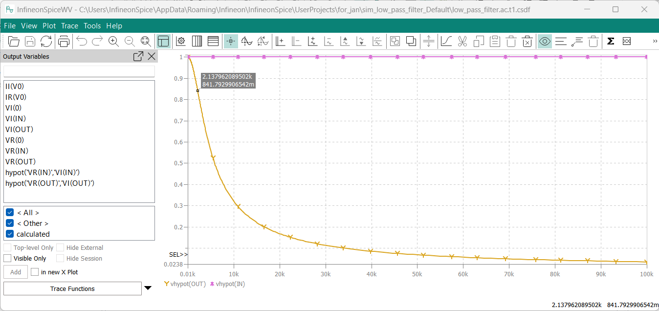
The plot shows the magnitudes of the IN and OUT signals.
Note that only the magnitudes for the IN and OUT signals were specified in the plot setup of the simulation. The real and imaginary values of the named voltages and currents of the schematic were automatically added in the
Output Variables
list.
Axes
When performing AC analyses with logarithmic range sweeps, you usually will want to switch the x-axes to logarithmic scaling by clicking

.
Traces
Some aspects of the signals that you can display as separate traces often have vastly different amplitudes than others, for example, attenuation or phase. You may want to display such traces in separate plots by choosing
.
Adding signal aspects
For any named signal in the schematic, the real and imaginary values are automatically added to the simulation. Other aspects – magnitude, attenuation, or phase – can be specified explicitly. If you have not done so when setting up the simulation, they can also be added later.
To do so, choose
in the Waveform Viewer window. This opens the
Freq Analysis
dialog:

Click the
Select
button and choose the desired signal. In the
Function
section, click the aspect that you want to add. A name and alias are automatically entered; you can edit them if desired.
From the
Place
list, choose the plot to which to add the trace. You can also specify that a new plot is created for the trace.
Finally, click
OK
to create the trace. The trace appears in the specified plot.